Quantum Computing for the Curious Developer: Building Your First Circuits with Qiskit
A developer's hands-on guide to quantum computing fundamentals — from qubits and gates to building a quantum teleportation circuit, no physics degree required.
You’ve read the headlines. Quantum computers will break encryption, revolutionize drug discovery, solve problems classical computers can’t touch. You’ve also tried to learn about them — and bounced off a wall of Dirac notation, Hilbert spaces, and physics jargon that assumes you already have a PhD.
I did too. Two years ago, I started a quantum computing project with Qiskit purely out of curiosity. The textbooks lost me. The IBM documentation felt like it was written for physicists. But somewhere between “what even is a qubit?” and building a working teleportation circuit, something clicked: quantum computing makes a lot more sense when you think like a developer, not a physicist.
This is Part 1 of a three-part series. By the end of this post, you’ll have built real quantum circuits — including one that teleports a quantum state from one qubit to another. No physics degree required. Just Python.
All code from this series is available in my quantum computing repository. The companion notebook for this post is here — you can follow along or run it directly.
Qubits: Bits That Haven’t Made Up Their Mind
A classical bit is either 0 or 1. A qubit is… also 0 or 1 when you look at it. The difference is what happens before you look.
Think of it like a coin. A classical bit is a coin lying on a table — heads or tails, always decided. A qubit is a coin mid-spin. It’s not heads and tails simultaneously — it exists in a superposition of both states, with probabilities for each outcome. The moment you “measure” the coin (catch it), it collapses to one definite result. And that collapse is irreversible — you can’t un-catch a coin to see how it was spinning.
Now let’s make that precise. Physicists write quantum states with bracket notation: means “the zero state” and means “the one state.” A qubit in superposition is written as:
Where and are numbers called amplitudes. They aren’t probabilities themselves, but they determine probabilities: when you measure, you get with probability and with probability . This is the Born rule — the bridge between the quantum world and the classical results we observe. Going back to the coin: the amplitudes describe how it’s spinning, and measurement forces it to land.
What’s Under the Hood
That and notation (called ket notation) is really just shorthand for column vectors:
A qubit in superposition is simply:
And here’s the part most tutorials skip: and can be complex numbers — they have both a real and an imaginary part (like ). The real part affects the magnitude, the imaginary part encodes the phase — a kind of hidden angle that doesn’t show up in measurement probabilities but matters when qubits interact through gates. Two states with the same and but different phases will behave differently when you apply gates to them. Phase is what makes quantum interference possible, and interference is what makes quantum algorithms work.
For this post, you won’t need to think about complex numbers — all our examples use real amplitudes. But when you see Qiskit output like Statevector([0.707+0.j, 0.707+0.j]), now you know: the +0.j is the imaginary part, and it’s zero.
Physically, a qubit is any quantum system with two distinguishable states — the spin of an electron (up or down), the polarization of a photon (horizontal or vertical), or in IBM’s quantum computers, a tiny superconducting circuit cooled to near absolute zero. We don’t need to worry about the physics. What matters for us as developers: you can’t peek at the amplitudes without destroying them, so you have to design circuits that manipulate them before measurement to get useful results out.
Getting Started
You’ll need Python and Qiskit v2. I have made a containerized setup, I have a Docker-based environment in the companion repository — just run make oci-build && make oci-run and you’ll have a Jupyter notebook ready to go. for which you just need to make oci-run
For running circuits on real quantum hardware, head to IBM Quantum Platform, sign up for a free account, and grab your API token. The free tier gives you 10 minutes of quantum compute time per month — more than enough to run everything in this post.
This post uses Qiskit v2.x. If you’re following along with older tutorials that use execute() or Aer.get_backend(), those are v1 patterns. The v2 API uses primitives (Sampler and Estimator) which we’ll cover below.
Now, let’s put a single qubit into superposition and measure it:
from qiskit import QuantumCircuit
from qiskit.primitives import StatevectorSampler

# 1 qubit, 1 classical bit to store the measurement
qc = QuantumCircuit(1, 1)
qc.h(0)            # Hadamard gate — puts qubit in superposition
qc.measure(0, 0)   # Measure the qubit

print(qc.draw())

sampler = StatevectorSampler()
result = sampler.run([qc], shots=1024).result()
counts = result[0].data['c'].get_counts()
print(counts)
# {'0': 489, '1': 535}  — roughly 50/50, as expected
That H in the circuit is the Hadamard gate — the most important gate in quantum computing. It takes a definite state and puts it into an equal superposition. When we measure, we get 0 or 1 with roughly equal probability. Run it again and you’ll get slightly different numbers. That’s not a bug — that’s quantum mechanics.
You can also build and visualize these circuits directly in IBM’s Quantum Composer. The Composer shows three visualization panels at the bottom of every circuit:
- Q-sphere (left): A 3D view of the multi-qubit quantum state in the computational basis (up to 5 qubits). Node size is proportional to the state’s probability, and color reflects the phase of each basis state.
- Statevector (center): The exact amplitudes of the quantum state across all computational basis states (up to 6 qubits). This completely characterizes the final output — it’s the theoretical “truth” before measurement noise.
- Probabilities (right): The likelihood of each measurement outcome across the computational basis states (up to 8 qubits). This is what you’d see if you ran the circuit on real hardware many times.
Here’s our Hadamard circuit in the Composer:

The Quantum Toolbox: Gates That Actually Matter
Classical computers have AND, OR, NOT gates. Quantum computers have their own set. You don’t need to memorize all of them, but three gates will get you surprisingly far:
X Gate (the NOT gate)
Flips to and vice versa. The quantum equivalent of a classical NOT.
qc = QuantumCircuit(1)
qc.x(0)  # Flip from |0⟩ to |1⟩
In the Composer, the Q-sphere dot moved from the top ( ) to the bottom ( ). The statevector flipped from to . The probability bar is now 100% on .
H Gate (Hadamard)
You’ve already seen this one. Takes a definite state and creates a superposition. Apply it again and it undoes the superposition — back to the original state. This reversibility is key to how quantum algorithms work.
CNOT Gate (Controlled-NOT)
This is where things get interesting. CNOT takes two qubits: a control and a target. If the control qubit is , it flips the target. If the control is , it does nothing. Sounds simple, but when the control qubit is in superposition, the CNOT gate creates entanglement.
qc = QuantumCircuit(2, 2)
qc.h(0)                              # Put qubit 0 in superposition
qc.cx(control_qubit=0, target_qubit=1)  # CNOT: entangle qubits
qc.measure([0, 1], [0, 1])

print(qc.draw())
This two-gate combo — Hadamard followed by CNOT — creates what’s called a Bell state. It’s the simplest entangled state and the building block for almost everything in quantum computing.

The Composer confirms it: the statevector is [1, 0, 0, 0] (before measurement normalization), and the probability panel shows only 00 and 11 — never 01 or 10.
Entanglement: The “Spooky” Part That’s Actually Simple
Entanglement has an intimidating reputation. Einstein called it “spooky action at a distance.” But from a developer’s perspective, it’s straightforward.
Let’s contrast two circuits. First, two independent qubits in superposition:
qc = QuantumCircuit(2, 2)
qc.h(0)  # Qubit 0 in superposition
qc.h(1)  # Qubit 1 in superposition (independently)
qc.measure([0, 1], [0, 1])

# Result: {'00': 244, '11': 265, '10': 248, '01': 243}
# All four outcomes — qubits are independent
Each qubit decides independently. You get all four combinations: 00, 01, 10, 11 — roughly 25% each.
Now, entangled qubits:
qc = QuantumCircuit(2, 2)
qc.h(0)
qc.cx(0, 1)  # CNOT creates entanglement
qc.measure([0, 1], [0, 1])

# Result: {'00': 510, '11': 514}
# ONLY 00 and 11 — qubits are correlatedOnly 00 and 11 appear. Never 01 or 10. The qubits are correlated — measuring one instantly tells you the other’s value. If qubit 0 is 0, qubit 1 is guaranteed to be 0. If qubit 0 is 1, qubit 1 is 1.
This isn’t the qubits communicating. It’s that the CNOT gate created a shared quantum state where these outcomes are the only possibilities. Think of it like tearing a playing card in half and mailing the pieces to two different cities — opening one envelope instantly tells you what the other person has. The information was encoded at the time of splitting, not at the time of opening.
The difference with quantum entanglement? The “card” was in superposition until one person opened their envelope. Einstein argued there must be hidden variables predetermining the outcomes — like the card halves already being decided. In 1964, physicist John Bell proved him wrong: no hidden variable theory can reproduce what quantum mechanics predicts. Experiments have since confirmed it. If you want the full story, Veritasium’s video on Bell’s theorem is the best explanation I’ve found.
Sampler vs Estimator: Two Ways to Read a Quantum Circuit
We’ve been using StatevectorSampler to run circuits and get histograms. But histograms aren’t the only way to extract information from a quantum circuit — and for understanding entanglement quantitatively, there’s something more powerful.
Qiskit gives you two primitives:
Sampler runs a circuit with measurements and gives you a histogram — “I ran this 1024 times, and got 00 510 times and 11 514 times.” It’s the intuitive one. You build a circuit, measure, count outcomes.
Estimator does something different. Instead of counting measurement outcomes, it calculates the expectation value of an observable — a single number that summarizes a specific physical property of your qubits. You don’t even put measure() gates in the circuit; the Estimator handles that internally.
What’s an Observable?
A qubit doesn’t have just one property you can check. You have to choose what to measure, like choosing between a ruler and a thermometer. In quantum computing, these “measurement tools” are called Pauli operators: Z, X, Y, and I.
- Z asks “are you or ?” — the standard measurement. Returns for , for .
- X asks “are you in the or superposition?” — measuring along a different axis.
- I means “ignore this qubit.”
For multiple qubits, you write strings of these. Qiskit reads them right to left, so "ZI" means “measure Z on qubit 1, ignore qubit 0.”
Proving Entanglement with Numbers
Remember the Bell state we just built — the one that only produced 00 and 11? The Sampler showed us that histogram. But the Estimator can tell us how correlated those qubits really are — and reveal something a histogram can’t.
Let’s measure three observables on our Bell state at once:
from qiskit import QuantumCircuit
from qiskit.quantum_info import SparsePauliOp
from qiskit.primitives import StatevectorEstimator

# The same Bell state circuit (no measurements needed for Estimator)
qc = QuantumCircuit(2)
qc.h(0)
qc.cx(0, 1)

# Three questions about our qubits:
obs_ZZ = SparsePauliOp("ZZ")  # "Do both qubits always agree?"
obs_ZI = SparsePauliOp("ZI")  # "Is qubit 1 biased towards 0 or 1?"
obs_IZ = SparsePauliOp("IZ")  # "Is qubit 0 biased towards 0 or 1?"

estimator = StatevectorEstimator()
result = estimator.run([(qc, [obs_ZZ, obs_ZI, obs_IZ])]).result()
print(result[0].data.evs)
# [1.0, 0.0, 0.0]| Observable | Ideal Value | Meaning |
|---|---|---|
ZZ | +1.0 | Qubits always agree — perfectly correlated |
ZI | 0.0 | Qubit 1 alone is completely random |
IZ | 0.0 | Qubit 0 alone is completely random |
That’s the beautiful paradox of entanglement: each qubit individually is perfectly random (ZI and IZ are zero — no bias whatsoever), but together they’re perfectly correlated (ZZ is 1.0 — they always agree). Neither qubit “knows” whether it’ll be 0 or 1, yet they always match.
When to use which? Use the Sampler when you care about the distribution of outcomes (histograms, probabilities). Use the Estimator when you care about a specific physical property (correlation, energy, magnetization). Most tutorials only show the Sampler — but the Estimator is what real quantum algorithms like VQE use under the hood to solve chemistry and optimization problems.
Here’s the same Estimator code running on real IBM hardware — the result [0.951, -0.018, 0.002] is close to the ideal [1.0, 0.0, 0.0]:
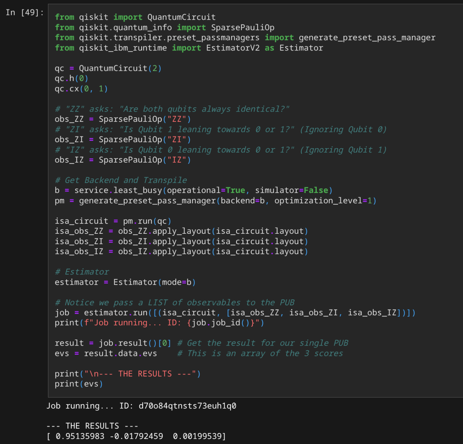
On a real IBM quantum computer, these values won’t be as clean. I ran this exact circuit on IBM hardware and got [0.951, -0.018, 0.002] — close to ideal, but noise from gate errors and decoherence degrades the results. IBM’s Runtime Estimator applies error mitigation that can even push values slightly outside the theoretical [-1, +1] range. We’ll dig into noise models and error mitigation in Part 3 of this series.
The Payoff: Quantum Teleportation in 20 Lines
Now for the part that made quantum computing click for me. We’re going to teleport a quantum state from one qubit to another. Not science fiction — a real protocol that IBM quantum computers execute every day.
Here’s the scenario: Alice has a qubit in some state she wants to send to Bob. They could be in different cities. She can’t just copy it — there’s a no-cloning theorem in quantum mechanics that makes copying an unknown quantum state physically impossible. But she can teleport it, if they share an entangled pair and a phone line.
The protocol has three acts. Let’s build it step by step.
Act 1: Setting the Stage
from qiskit import QuantumCircuit
from qiskit_aer import AerSimulator

qc = QuantumCircuit(3, 3)

# Alice prepares the state she wants to teleport on qubit 0
qc.x(0)   # Flip to |1⟩
qc.z(0)   # Apply a phase flip → now it's -|1⟩
qc.barrier()
We have three qubits: q0 is Alice’s secret state (the one she wants to teleport), q1 will be Alice’s half of the entangled pair, and q2 is Bob’s half. Right now only q0 has been touched — Alice has prepared it in the state using X and Z gates.
Act 2: The Shared Entangled Pair
# Create a Bell pair between qubits 1 and 2
qc.h(1)
qc.cx(1, 2)
qc.barrier()
Before Alice and Bob separated, they created an entangled pair — the same H + CNOT Bell state we built earlier. Alice keeps q1, Bob takes q2 to his city. They’re now correlated: measuring one instantly determines the other.
At this point, Alice has two qubits (q0 with her secret state, q1 as her entangled half) and Bob has one qubit (q2).
Act 3: The Teleportation
Here’s where it gets clever. Alice can’t look at her secret state (measuring it would destroy the superposition). Instead, she entangles her secret qubit with her half of the pair, then measures both of her qubits.
# Alice entangles her secret state (q0) with her half of the pair (q1)
qc.cx(0, 1)   # CNOT: transfers information about q0 into the entangled pair
qc.h(0)       # Hadamard: spreads the information across both measurement outcomes

# Alice measures her two qubits and calls Bob with the results
qc.measure(0, 0)
qc.measure(1, 1)
Why does this work? The CNOT + H combination “encodes” Alice’s secret state into the correlations of the entangled pair. Alice’s measurement collapses her qubits into one of four random outcomes (00, 01, 10, or 11) — but each outcome leaves Bob’s qubit in a specific state that’s related to the original. Alice’s measurement result tells Bob exactly which corrections to apply.
# Bob applies corrections based on Alice's measurement results
# If Alice's q1 measured 1 → Bob applies X gate
qc.cx(1, 2)
qc.barrier()In a real-world scenario, Alice would phone Bob and say “I got 01” or “I got 10”, and Bob would apply the corresponding correction gates. In our circuit, Qiskit handles this with classical conditioning — the cx(1, 2) after measurement uses Alice’s classical bit to control Bob’s gate. This is why teleportation doesn’t break physics: it requires classical communication (limited to the speed of light) to complete.
Verifying It Worked
How do we prove the teleportation happened? We reverse the original preparation on Bob’s qubit. If his qubit truly received Alice’s state (), then applying Z then X (the reverse of X then Z) should return it cleanly to .
# Undo Alice's original preparation on Bob's qubit
qc.z(2)   # Reverse the Z
qc.x(2)   # Reverse the X → should be back to |0⟩
qc.measure(2, 2)
Let’s run it:
simulator = AerSimulator()
result = simulator.run(qc, shots=1024).result()
print(result.get_counts())
# {'001': 253, '010': 254, '000': 253, '011': 264}
Look at qubit 2 (the leftmost bit in Qiskit’s little-endian convention). It’s always 0. The outcomes are 000, 001, 010, 011 — Bob’s bit never flips to 1. After reversing the preparation, Bob’s qubit returned to . The teleportation worked.
Alice’s two bits (positions 0 and 1) are random — that’s expected. She gets one of four equally likely outcomes each run. But regardless of which outcome she gets, Bob’s qubit always ends up with her original state.
The Full Circuit
Three barriers, three acts. State preparation, shared entanglement, teleportation. Twenty lines of code to move a quantum state without copying it — something Einstein didn’t believe was possible.
Here’s the full circuit in IBM’s Quantum Composer — the Q-sphere and probability panels confirm the teleportation:

But What About Arbitrary States?
Teleporting and is cool, but the real power of teleportation is moving any qubit state — a qubit rotated to 60 degrees, or some messy superposition that you can’t even describe classically. Can we see that?
Yes. But first, a confession: our circuit above was incomplete. It only had one correction gate (cx(1,2)), which happened to work for the specific state. For an arbitrary state, Bob actually needs two corrections:
cx(1, 2)— if Alice’s q1 measured 1, flip Bob’s qubit (X correction)cz(0, 2)— if Alice’s q0 measured 1, fix the phase (Z correction)
Why specifically X and Z? After Alice measures, the math shows Bob’s qubit lands in one of four states depending on Alice’s outcome:
| Alice measures | Bob’s qubit | Correction |
|---|---|---|
| 00 | None — already correct | |
| 01 | X — amplitudes are swapped, flip them back | |
| 10 | Z — sign is wrong, fix the phase | |
| 11 | XZ — both errors, apply both corrections |
Two types of errors, two independent corrections. Alice’s q1 bit controls X (bit flip), Alice’s q0 bit controls Z (phase flip). That’s why cx and cz — each conditioned on a different classical bit. No Y gate needed: , and that global phase doesn’t affect measurements.
Let’s teleport a qubit rotated by 60 degrees. First, let’s see exactly what state Alice is sending. The ry(π/3) gate creates the state . We can inspect the exact statevector using Statevector.from_instruction() — Qiskit’s way to get the theoretical state of a circuit without running any simulation:
from qiskit import QuantumCircuit
from qiskit_aer import AerSimulator
from qiskit.quantum_info import Statevector
from qiskit.visualization import plot_bloch_multivector, plot_histogram
from math import pi

theta = pi / 3  # 60 degrees

# Alice's exact state — no simulator needed
qc_alice = QuantumCircuit(1)
qc_alice.ry(theta, 0)
alice_state = Statevector.from_instruction(qc_alice)
alice_probs = alice_state.probabilities()
print("Alice's state:", alice_state)
print(f"Probabilities: |0⟩ = {alice_probs[0]:.4f}, |1⟩ = {alice_probs[1]:.4f}")
# Alice's state: Statevector([0.8660254+0.j, 0.5+0.j])
# Probabilities: |0⟩ = 0.7500, |1⟩ = 0.2500
Alice’s statevector is . By the Born rule, the probability of each outcome is the amplitude squared — so 75% chance of and 25% chance of . If teleportation works, Bob’s qubit should show that exact same 75/25 split.
Now let’s teleport it with both corrections:
qc = QuantumCircuit(3, 3)
qc.ry(theta, 0)
qc.barrier()

qc.h(1)
qc.cx(1, 2)
qc.barrier()

qc.cx(0, 1)
qc.h(0)
qc.measure(0, 0)
qc.measure(1, 1)

# Bob's corrections — BOTH needed for arbitrary states
qc.cx(1, 2)   # X correction based on Alice's q1
qc.cz(0, 2)   # Z correction based on Alice's q0
qc.barrier()

qc.measure(2, 2)

simulator = AerSimulator()
result = simulator.run(qc, shots=4096).result()
counts = result.get_counts()

# Extract Bob's qubit (leftmost bit in Qiskit's convention)
bob_0 = sum(v for k, v in counts.items() if k[0] == '0')
bob_1 = sum(v for k, v in counts.items() if k[0] == '1')
total = bob_0 + bob_1

print(f"Alice's probs:   |0⟩ = {alice_probs[0]:.4f}, |1⟩ = {alice_probs[1]:.4f}")
print(f"Bob's measured:  |0⟩ = {bob_0/total:.4f}, |1⟩ = {bob_1/total:.4f}")
# Alice's probs:   |0⟩ = 0.7500, |1⟩ = 0.2500
# Bob's measured: |0⟩ = 0.7456, |1⟩ = 0.2544| Alice (theoretical) | 0.7500 | 0.2500 |
| Bob (simulator) | 0.7456 | 0.2544 |
| Bob (real IBM hardware) | 0.7297 | 0.2703 |
The simulator is nearly perfect — the tiny difference is just shot noise from sampling. The real IBM quantum computer is only ~2% off from ideal. Noise from gate errors and decoherence pushes the results slightly toward 50/50 (randomness), but the 75/25 signal comes through clearly. The teleportation preserved the full quantum state, not just a classical 0 or 1.
Try changing theta to different angles. At (90°) you’ll get a perfect 50/50 split. At (45°) you’ll get roughly 85/15. The ratio always matches to — proof that the entire quantum state is being teleported, not just a bit.
The gap between simulator and real hardware is small here, but it grows with circuit complexity. Understanding why real qubits are noisy and how to mitigate those errors is the subject of Part 3 in this series.
Where to Go From Here
Two years ago, I started with a QuantumCircuit(2, 2) and a vague understanding of superposition. The moment I saw teleportation actually work — Bob’s qubit consistently returning the right state, verified against real IBM hardware — was when quantum computing stopped being abstract physics and started being engineering.
Here’s what we covered:
- Qubits live in superposition until measured — then they collapse
- Three gates get you surprisingly far: H (superposition), X (NOT), CNOT (entanglement)
- Entanglement makes qubits individually random but collectively correlated
- Sampler gives you histograms; Estimator gives you physical properties — both are essential
- Teleportation transfers a complete quantum state using entanglement, proven on both simulator and real hardware
The circuits we built today are the foundation for everything that comes next. In Part 2, we’ll see why quantum computing actually matters: algorithms that provably outperform classical computers. Deutsch’s algorithm, Grover’s search, and the one that keeps cryptographers up at night — Shor’s factoring algorithm.
The secret I wish someone had told me at the start: you don’t need to understand the math to build the intuition. Write the circuit. Run it. Look at the histogram. Then the math starts making sense.

Other posts
See all posts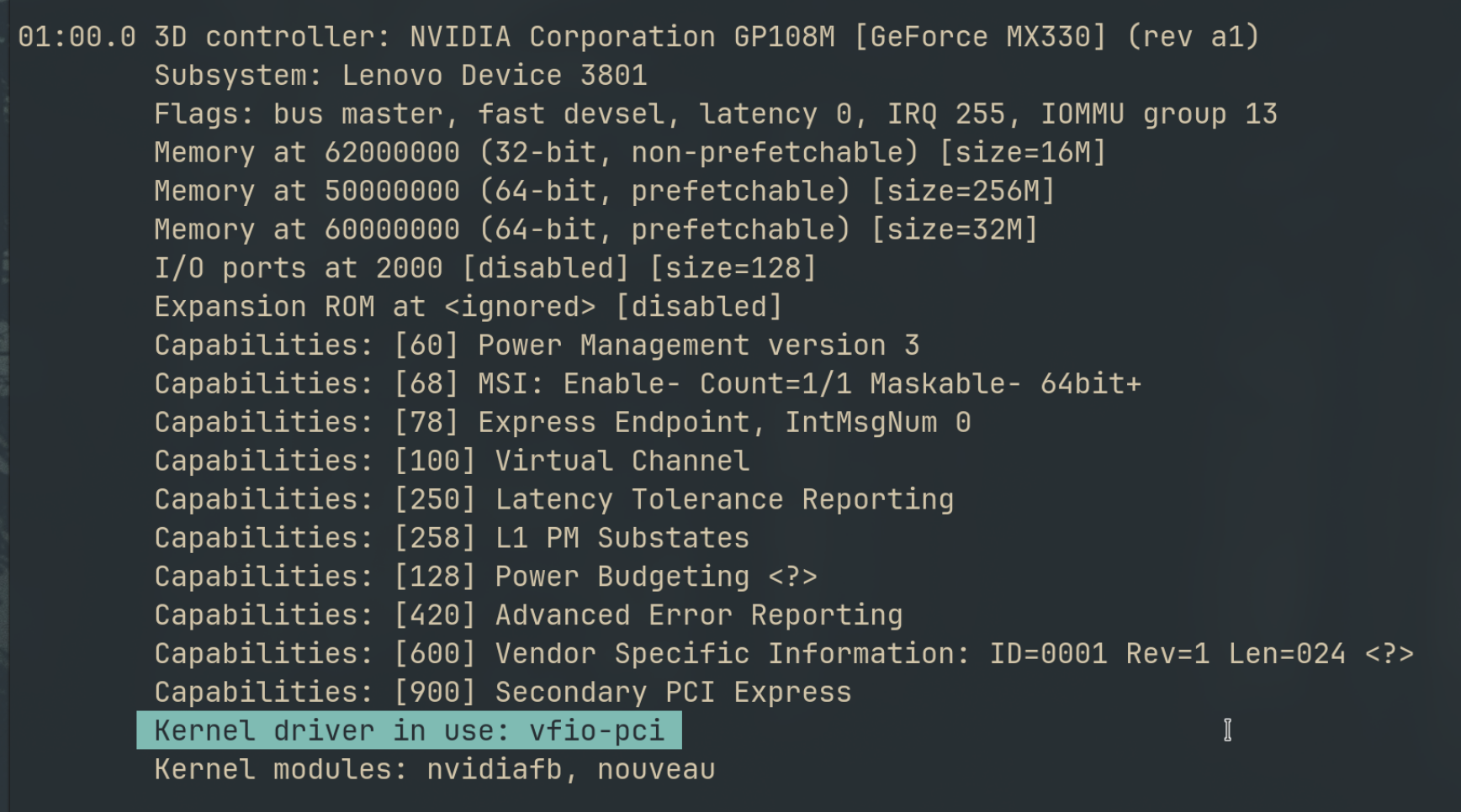
Why Your Laptop GPU Will Never Work with Proxmox Passthrough
Six attempts, three days, one stubborn MX330. A post-mortem on laptop GPU passthrough in Proxmox — what failed, why it's architecturally impossible, and exactly what to buy instead.

Your Old Laptop Is a Linux Server: A Complete Proxmox Home Lab Setup Guide
Turn an old laptop into a full Proxmox home server — Wi-Fi NAT routing, DHCP, MTU fixes, and every gotcha you'll actually hit. A practical guide that also teaches you how AWS works.
When localhost Lied to Me: Debugging Playwright in a Containerized CI Runner
A Docker networking war story — why localhost lies inside containers, how --add-host gets you close, and how socat bridges the final gap for Playwright E2E tests.